In this post we are going to discuss how we can predict the weekly candle high, low and close for this week on Monday morning. Did you watch the video on the day in the life of a millionaire forex trader? Trading is all about reducing the risk as much as possible. I had started trading with a stop loss of 50 pips. With the passage of time, I improved my strategy and now I mostly trade with a stop loss of 10-20 pips. My profit target is always 100-200 pips. So you can see almost all the trades that I make have a reward/risk ratio of at least 5:1. Risk management is the most important thing in trading.
In this post we are going to discuss how we can use neural networks in making our trading system more accurate. If we can accurately predict the weekly candle high, low and close this can improve our trading accuracy. Did you read the post on how to make 200 pips with a small stop loss of 10 pips? In this post I explained how just by using candlesticks we can achieve a low risk and high reward performance. Now this is what we want to do. We want to predict the shape of the weekly candle so that we know what will be the high, low and close of the weekly candle. We already know the open. We will be using 2 different neural network algorithms in calculating the weekly candle high, low and close. If both algorithms give almost similar predictions we can accept the predictions. On the other hand if both algorithms differ than we should not accept the prediction. We will be using NNET and NeuralNet packages from R. We hope you have R software installed on your computer and you know how to import the data into R and make the calculations. Did you download the Pin Bar Indicator FREE? So let’s start.
Weekly High, Low and Close Prediction Using NeuralNet Algorithm
First we will use the NeuralNet R package for calculating the weekly high, low and close.
> #predict the weekly close
>
> #import the data
>
> data <- read.csv("E:/MarketData/GBPUSD10080.csv", header = FALSE)
>
> colnames(data) <- c("Date", "Time", "Open", "High",
+                     "Low", "Close", "Volume")
>
> library(quantmod)
>
> data2 <- as.xts(data[,-(1:2)], as.Date(paste(data[,1]),format='%Y.%m.%d'))
>
>
> data2$rsi <- RSI(data2$Close)
> data2$MACD <- MACD(data2$Close)
> data2$will <- williamsAD(data2[,2:4])
> data2$cci <-  CCI(data2[,2:4])
> data2$STOCH <- stoch(data2[,2:4])
> data2$Aroon <- aroon(data2[, 2:3])
> data2$ATR <- ATR(data2[, 2:4])
>
>
>
> data2$Return <- diff(log(data2$Close))
>
>
>
> x <- nrow(data2)
> y <- ncol(data2)
>
> for (i in (x-1000):(x-1))
+ {
+
+   data2[i,y] <- data2[i+1,y]
+
+
+ }
>
>
>
>
> library("neuralnet")
>
> f <-Return~ Open+High+Low+Close+Volume+rsi+macd+
+   MACD+will+cci+fastK+fastD+STOCH+aroonUp+aroonDn+
+   Aroon+tr+atr+trueHigh+ATR
>
> fitM <- neuralnet (f,
+                    data = data2[(x-1000):(x-2), 1:y],
+                    hidden =c(15 ,15) ,
+                    stepmax = 25000 ,
+                    algorithm = "rprop+",
+                    err.fct = "sse",
+                    act.fct = "logistic",
+                    rep =10 ,
+                    linear.output = FALSE )
>
>
> ## predict the next candle
>
>
>
> pred <- compute(fitM , data2[x-1, 1:y-1])
>
> pred$net.result
                     [,1]
2016-09-25 0.001291996305
>
>
>
> exp(pred$net.result)*data[x-1,6]
                  [,1]
2016-09-25 1.299678095
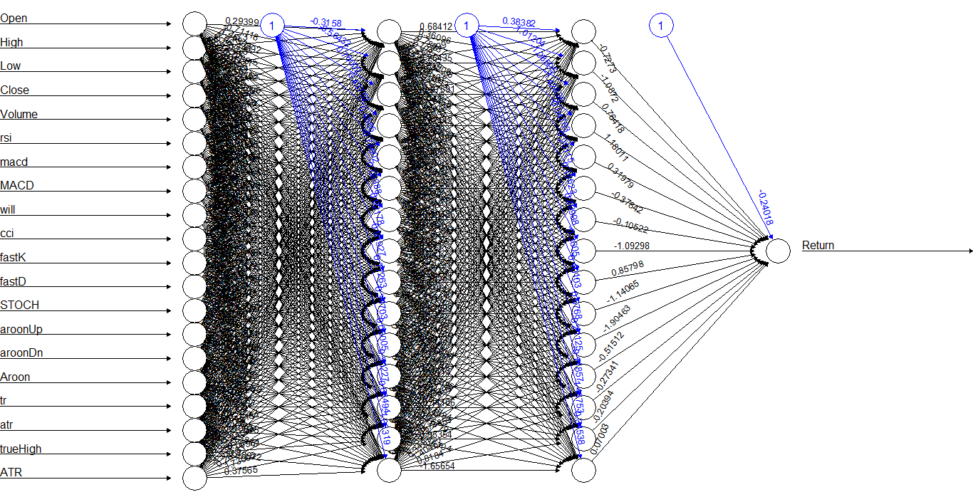
As you can see above, predicted weekly close is 1.2996. Below is a plot of the neural net that was used in the calculations. You can see in the plot below the total number of inputs used were 20 that included open, high, low, close, volume,rsi,macd,MACD, will, cci STOCH, Aroon, ATR etc. NeuralNet R package is pretty fast and it finished the calculations in a few seconds. Next we calculate the weekly high.
> #predict the weekly high
> #import the data
>
> data <- read.csv("E:/MarketData/GBPUSD10080.csv", header = FALSE)
>
> colnames(data) <- c("Date", "Time", "Open", "High",
+                     "Low", "Close", "Volume")
>
> library(quantmod)
>
> data2 <- as.xts(data[,-(1:2)], as.Date(paste(data[,1]),format='%Y.%m.%d'))
>
>
> data2$rsi <- RSI(data2$High)
> data2$MACD <- MACD(data2$High)
> data2$will <- williamsAD(data2[,2:4])
> data2$cci <-  CCI(data2[,2:4])
> data2$STOCH <- stoch(data2[,2:4])
> data2$Aroon <- aroon(data2[, 2:3])
> data2$ATR <- ATR(data2[, 2:4])
>
>
>
> data2$Return <- diff(log(data2$High))
>
>
>
> x <- nrow(data2)
> y <- ncol(data2)
>
> for (i in (x-1000):(x-1))
+ {
+
+   data2[i,y] <- data2[i+1,y]
+
+
+ }
>
>
>
>
> library("neuralnet")
>
> f <-Return~ Open+High+Low+Close+Volume+rsi+macd+
+   MACD+will+cci+fastK+fastD+STOCH+aroonUp+aroonDn+
+   Aroon+tr+atr+trueHigh+ATR
>
> fitM <- neuralnet (f,
+                    data = data2[(x-1000):(x-2), 1:y],
+                    hidden =c(15 ,15) ,
+                    stepmax = 25000 ,
+                    algorithm = "rprop+",
+                    err.fct = "sse",
+                    act.fct = "logistic",
+                    rep =10 ,
+                    linear.output = FALSE )
>
>
> ## predict the next candle
>
>
>
> pred <- compute(fitM , data2[x-1, 1:y-1])
>
> pred$net.result
                      [,1]
2016-09-25 0.0004830697142
>
>
>
> exp(pred$net.result)*data[x-1,4]
                  [,1]
2016-09-25 1.306500979
The predicted weekly high is 1.3065. Next we calculate the weekly low.
> #predict the weekly low
>
> #import the data
>
> data <- read.csv("E:/MarketData/GBPUSD10080.csv", header = FALSE)
>
> colnames(data) <- c("Date", "Time", "Open", "High",
+                     "Low", "Close", "Volume")
>
> library(quantmod)
>
> data2 <- as.xts(data[,-(1:2)], as.Date(paste(data[,1]),format='%Y.%m.%d'))
>
>
> data2$rsi <- RSI(data2$Low)
> data2$MACD <- MACD(data2$Low)
> data2$will <- williamsAD(data2[,2:4])
> data2$cci <-  CCI(data2[,2:4])
> data2$STOCH <- stoch(data2[,2:4])
> data2$Aroon <- aroon(data2[, 2:3])
> data2$ATR <- ATR(data2[, 2:4])
>
>
>
> data2$Return <- diff(log(data2$Low))
>
>
>
> x <- nrow(data2)
> y <- ncol(data2)
>
> for (i in (x-1000):(x-1))
+ {
+
+   data2[i,y] <- data2[i+1,y]
+
+
+ }
>
>
>
>
> library("neuralnet")
>
> f <-Return~ Open+High+Low+Close+Volume+rsi+macd+
+   MACD+will+cci+fastK+fastD+STOCH+aroonUp+aroonDn+
+   Aroon+tr+atr+trueHigh+ATR
>
> fitM <- neuralnet (f,
+                    data = data2[(x-1000):(x-2), 1:y],
+                    hidden =c(15 ,15) ,
+                    stepmax = 25000 ,
+                    algorithm = "rprop+",
+                    err.fct = "sse",
+                    act.fct = "logistic",
+                    rep =10 ,
+                    linear.output = FALSE )
>
>
> ## predict the next candle
>
>
>
> pred <- compute(fitM , data2[x-1, 1:y-1])
>
> pred$net.result
                     [,1]
2016-09-25 0.001978147771
>
>
>
> exp(pred$net.result)*data[x-1,5]
                  [,1]
2016-09-25 1.294197584
Predicted weekly low is 1.2941.
Weekly High, Low and Close Prediction Using NNET Algorithm
Now let’s do the same calculations using NNET algorithm. This algorithm is different from NeuralNet algorithm. the inputs will be the same but the algorithm will be different. NNET is a single layer perceptron whereas NeuralNet is a multilayer perceptron. What we want to compare the predictions made from the 2 algorithms. So let’s start.
> #predict the close for the week
> #import the data
>
> data <- read.csv("E:/MarketData/GBPUSD10080.csv", header = FALSE)
>
> colnames(data) <- c("Date", "Time", "Open", "High",
+                     "Low", "Close", "Volume")
>
> library(quantmod)
>
> data2 <- as.xts(data[,-(1:2)], as.Date(paste(data[,1]),format='%Y.%m.%d'))
>
>
>
> data2$rsi <- RSI(data2$Close)
> data2$MACD <- MACD(data2$Close)
> data2$will <- williamsAD(data2[,2:4])
> data2$cci <-  CCI(data2[,2:4])
> data2$STOCH <- stoch(data2[,2:4])
> data2$Aroon <- aroon(data2[, 2:3])
> data2$ATR <- ATR(data2[, 2:4])
>
>
> data2$Return <- diff(log(data2$Close))
>
>
> x <- nrow(data2)
>
> for (i in (x-1000):(x-1))
+ {
+
+   data2[i,21] <- data2[i+1,21]
+
+
+ }
>
>
>
> library(nnet)
> fit1 <- nnet( Return~ Open+High+Low+Close+Volume+rsi+macd+
+                 MACD+will+cci+fastK+fastD+STOCH+aroonUp+aroonDn+
+                 Aroon+tr+atr+trueHigh+ATR,
+               data = data2[(x-1000):(x-2), 1:21], maxit = 5000,
+               size = 20, decay = 0.01, linout = 1, trace=F)
> pred <- predict(fit1, newdata = data2[x-1, 1:20])
>
>
> exp(pred[1])*data[x-1,6]
[1] 1.296095126
The weekly close predicted by NNET algorithm is 1.2960 while that predicted by NeuralNet algorithm is 1.2996. There is not much difference. Next we predict the weekly high.
> #predict the high for the week
>
> #import the data
>
> data <- read.csv("E:/MarketData/GBPUSD10080.csv", header = FALSE)
>
> colnames(data) <- c("Date", "Time", "Open", "High",
+                     "Low", "Close", "Volume")
>
> library(quantmod)
>
> data2 <- as.xts(data[,-(1:2)], as.Date(paste(data[,1]),format='%Y.%m.%d'))
>
>
>
> data2$rsi <- RSI(data2$High)
> data2$MACD <- MACD(data2$High)
> data2$will <- williamsAD(data2[,2:4])
> data2$cci <-  CCI(data2[,2:4])
> data2$STOCH <- stoch(data2[,2:4])
> data2$Aroon <- aroon(data2[, 2:3])
> data2$ATR <- ATR(data2[, 2:4])
>
>
> data2$Return <- diff(log(data2$High))
>
>
> x <- nrow(data2)
>
> for (i in (x-1000):(x-1))
+ {
+
+   data2[i,21] <- data2[i+1,21]
+
+
+ }
>
>
>
> library(nnet)
> fit1 <- nnet( Return~ Open+High+Low+Close+Volume+rsi+macd+
+                 MACD+will+cci+fastK+fastD+STOCH+aroonUp+aroonDn+
+                 Aroon+tr+atr+trueHigh+ATR,
+               data = data2[(x-1000):(x-2), 1:21], maxit = 5000,
+               size = 20, decay = 0.01, linout = 1, trace=F)
> pred <- predict(fit1, newdata = data2[x-1, 1:20])
>
>
> exp(pred[1])*data[x-1,4]
[1] 1.310862369
The weekly high predicted by NNET algorithm is 1.3108 while that predicted by NeuralNet is 1.3065. There is a difference of 40 pips.
> #predict the low for thw week
>
>
> #import the data
>
> data <- read.csv("E:/MarketData/GBPUSD10080.csv", header = FALSE)
>
> colnames(data) <- c("Date", "Time", "Open", "High",
+                     "Low", "Close", "Volume")
>
> library(quantmod)
>
> data2 <- as.xts(data[,-(1:2)], as.Date(paste(data[,1]),format='%Y.%m.%d'))
>
>
>
> data2$rsi <- RSI(data2$Low)
> data2$MACD <- MACD(data2$Low)
> data2$will <- williamsAD(data2[,2:4])
> data2$cci <-  CCI(data2[,2:4])
> data2$STOCH <- stoch(data2[,2:4])
> data2$Aroon <- aroon(data2[, 2:3])
> data2$ATR <- ATR(data2[, 2:4])
>
>
> data2$Return <- diff(log(data2$Low))
>
>
> x <- nrow(data2)
>
> for (i in (x-1000):(x-1))
+ {
+
+   data2[i,21] <- data2[i+1,21]
+
+
+ }
>
>
>
> library(nnet)
> fit1 <- nnet( Return~ Open+High+Low+Close+Volume+rsi+macd+
+                 MACD+will+cci+fastK+fastD+STOCH+aroonUp+aroonDn+
+                 Aroon+tr+atr+trueHigh+ATR,
+               data = data2[(x-1000):(x-2), 1:21], maxit = 5000,
+               size = 12, decay = 0.01, linout = 1, trace=F)
> pred <- predict(fit1, newdata = data2[x-1, 1:20])
>
>
> exp(pred[1])*data[x-1,5]
[1] 1.291337137
The predicted weekly low by NNET package is 1.2913 while that by NeuralNet package is 1.2940. So we have a rough idea of the shape of the weekly candle. We will now use this knowledge in making better trading decisions. Did you read the post on how to trade on M30 and double your account?